The Dangers of Performance Metrics

Full disclosure: I’m not a big fan of one-dimensional metrics when evaluating (binary) classifiers (e.g. a neural network that is supposed to distinguish pictures of cats and dogs). In my opinion, a confusion matrix is, in almost all instances, preferable for data scientists. However, that doesn’t mean there aren’t good reasons to use one-dimensional performance metrics:

• They are (deceptively) simple,
• Easy to integrate in cross validation and similar automated processes,
• Can be an excellent communication tool,
• …

My gripe with performance metrics is founded in the observation that they tend to be footguns in practice – outside of the academical environment they’ve been born it:

• Their actual expressive power often isn’t clear,
• It’s remarkably common for people to chase metrics that don’t align with their goals,
• The terminology can be misleading ¹ and
• Choosing a metric is often less a result of careful consideration than a symptom of information bias or high uncertainty avoidance.

Note that none of these points has to do with performance metrics as mathematical concepts – they are instances of human misconduct. Therefore, instead of continuing my crusade against the status quo, I’d like to take a few minutes to discuss some common metrics and how/when you should pay and, more importantly, when you should not pay attention to them.

Black or True Black?

Before we can hope to understand common performance metrics we need to talk about True Positives and True Negatives.

CS8k at work

Suppose we have a binary classifier, call it ‘CatSniffer8000’ (CS8k), that is supposed to tell us whether a given picture shows a cat or not. We have a test dataset of 1000 pictures, exactly 400 of which show cats, that we ask CS8k to classify. And we end up with the following confusion matrix:

CS8k's confusion matrix

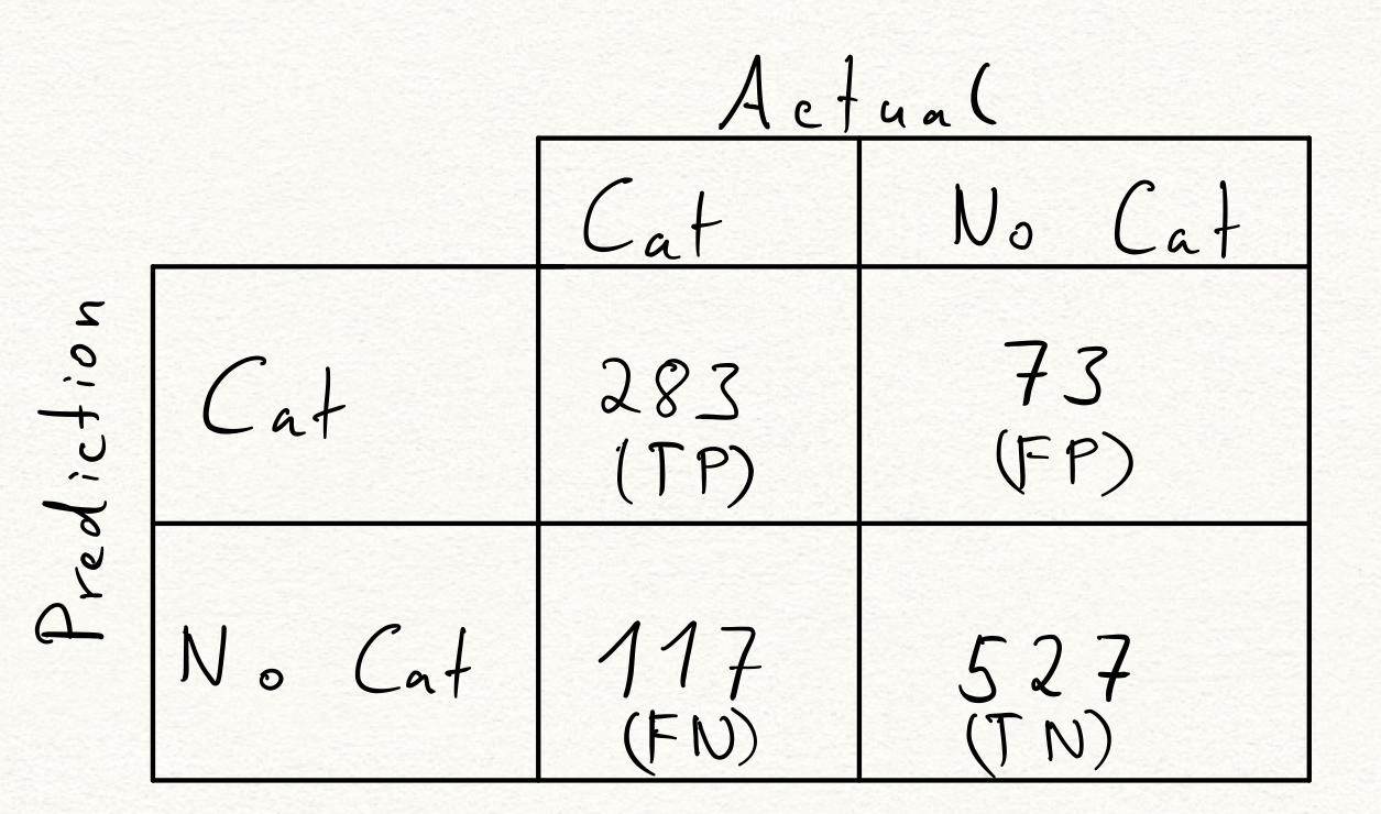
There are 400 cat pictures in our training set. These are the Positives (P). And, likewise, there are 600 pictures that don’t show cats – the Negatives (N).

Out of the 400 pictures that showed cats (our Positives), CS8k correctly labelled 283 as cats. These are the True Positives (TP). In other words: True Positives are those instances that are labelled as positive both in our training set and by our classifier.

Similarly, out of 600 pictures in our training set that didn’t show cats, CS8k correctly labelled 527 as ‘non cats’. These are the True Negatives (TN).

Furthermore, 73 non-cat pictures got incorrectly labelled as cat picture. This amounts to 73 False Positives (FP).

Finally, 117 cat pictures in our dataset received the label ‘no cat’ by CS8k – resulting in 117 False Negatives (FN).

Note that always

#Negatives = #True Negatives + #False Positives and

#Positives = #True Positives + #False Negatives.

This is a good sanity check when filling out a confusion matrix (or interpreting an unlabelled one).

Accuracy, Recall, Precision and F1-Score

Now that we know about True/False Positives/Negatives, we can use them to define common performance metrics.

Accuracy

The one pretty much everyone will have seen is Accuracy (ACC). It’s defined as

\[ \mathrm{ACC} = \frac{\mathrm{TP} + \mathrm{TN}}{\mathrm{P} + \mathrm{N}} \]

but what does it mean? Well, it’s the ratio of all instances that have been labelled correctly by our classifier. As such is serves as a good default performance metric for many tasks – especially if the test set is balanced (i.e. \(\mathrm{P}\) and \(\mathrm{N}\) are of similar size) and consists of groups of roughly equal importance to your task.

The accuracy of CS8k is \(\frac{283+527}{400 + 600} = 0.81 = 81 \%\).

Let’s consider an example in which accuracy is a terrible metric: Suppose you decide to build a model that tries to detect breast cancer in women from their X-ray images. Your dataset consists of 100.000 randomly selected images and, as such, only contains 85 Positives. By always guessing ‘not breast cancer’, your classifier will achieve an accuracy of \(\frac{0 + 99.015}{100000} = 99.015\%\). And despite this impressive performance metric, you hopefully agree with me that this is an absolutely terrible model.

Recall

To mathematically capture the awfulness of our breast cancer classifier, we should look at its Recall or True Positive Rate (TPR). It’s defined as

\[ \mathrm{TPR} = \frac{\mathrm{TP}}{P} \]

and hence turns out to be a whopping \(\frac{0}{85} = 0\%\) – truly awful!

Recall measures how many of the Positives got detected as such and only that. While it can be a highly relevant piece of information, it is not suitable as your single performance metric. By blindly guessing ‘Positive’, your model will always have a Recall of \(100\%\).

Precision

Contrary to Recall, Precision or Positive Predictive Value (PPV) measures the ratio of Positives among all those instances that our classifier labelled as positive.

\[ \mathrm{PPV} = \frac{\mathrm{TP}}{\mathrm{TP} + \mathrm{FP}} \]

Since \(\mathrm{FP} = 0\) for our breast cancer classifier, it has perfect precision – demonstrating that precision alone also isn’t suitable as a performance metric.

F1 Score

This is where the F1-Score (F1) comes into play. It’s the harmonic mean of Recall and Precision which makes is much more useful as a performance metric than either of its building blocks. The precise mathematical definition is

\[ \mathrm{F1} = \frac{2}{\frac{1}{\mathrm{TPR}} + \frac{1}{\mathrm{PPV}}} = \frac{2 \cdot \mathrm{TP}}{2 \cdot \mathrm{TP} + \mathrm{FP} + \mathrm{FN}}. \]

In order to achieve a high F1-Score, your model must achieve both high Recall and Precision ². Not only that, because of the usage of the harmonic mean, a terrible score in either metric will destroy the F1-Score. In particular, our breast cancer classifier, despite having perfect precision, has an F1-Score of \(\frac{2 \cdot 0}{ 2 \cdot 0 + 0 + 85} = 0\).

If your task demands a balance of Recall and Precision (which typically require trade-offs), the F1-Score is a decent choice. However, it’s not a silver bullet for your performance metric needs either:

Consider the following scenario: We keep everything as before but flip the labels in our breast cancer example. So the breast cancer instances are now our Negatives and the non-breast cancer instances are now our Positives. Having changed nothing about the quality of our model, this now results in an F1-Score of \(\frac{2 \cdot 99.015}{2 \cdot 99.0815 + 85 + 0 } \sim 0.9996\) – a nearly perfect score.

There are other issues with these and every other one-dimensional performance metric but I think I’ve already demanded too much of your attention for now. So let’s reserve further criticism for another time…

Recommended Default

Let me stress again that metrics are neither good or bad. If handled responsibly, they’re powerful tools for data scientists and disregarding their value would be a foolish move. However, as I’ve tried to argue in this post, I do think that metrics should guide your decision making only after careful evaluation of their appropriateness for the task at hand. I’m not kidding when I’m saying that, in practice, metrics tend to be footguns. It’s incredibly easy to misinterpret what a given score/value means in your particular case and how it should (or shouldn’t) affect your decisions.

In fact, I’d go as far as to say that the default for data science practitioners should be to not consider any one-dimensional metric and instead analyse confusion matrices. They are, without a doubt, less convenient but that actually turns out to be their strength: Being forced to carefully thing through a confusion matrix will save your from making many mistakes that looking at a single, poorly chosen performance metric alone would have nudged you to commit.

1. Metrics tend to have names that we attach some intuitive meaning to (like ‘accuracy’) that doesn’t always align with the technical definition. ↩

2. Not that, although the F1-Score takes only values between 0 and 1, people don’t often view the F1-Score as a percentage. And there are good reasons for that, that I won’t get into here. ↩